2. Getting Started with Conx

2.1. What is conx?

Conx is an accessible and powerful way to build and understand deep learning neural networks. Specifically, it sits on top of Keras, which sits on top of Theano, TensorFlow, or CNTK.

Conx:

• has an easy to use interface for creating connections between layers of a neural network
• adds additional functionality for manipulating neural networks
• supports visualizations and analysis for training and using neural networks
• has everything you need; doesn’t require knowledge of complicated numerical or plotting libraries
• integrates with lower-level (Keras) if you wish

But rather than attempting to explain each of these points, let’s demonstrate them.

This demonstration is being run in a Jupyter Notebook. Conx doesn’t require running in the notebook, but if you do, you will be able to use the visualizations and dashboard.

2.2. A Simple Network

As a demonstration, let’s build a simple networkd for learning the XOR (exclusive or) truth table. XOR is defined as:

Input 1	Input 2	Output
0	0	0
0	1	1
1	0	1
1	1	0

2.2.1. Step 1: import conx

We will need the Network, and Layer classes from the conx module:

import conx as cx

Using TensorFlow backend.
Conx, version 3.6.0

2.2.2. Step 2: create the network

Every network needs a name:

net = cx.Network("XOR Network")

2.2.3. Step 3: add the needed layers

Every layer needs a name and a size. We add each of the layers of our network. The first layer will be an “input” layer (named “input1”). We only need to specify the size. For our XOR problem, there are two inputs:

net.add(cx.Layer("input1", 2))

'input1'

For the next layers, we will also use the default layer type for hidden and output layers. However, we also need to specify the function to apply to the “net inputs” to the layer, after the matrix multiplications. We have a few choices for which activation functions to use:

• ‘relu’
• ‘sigmoid’
• ‘linear’
• ‘softmax’
• ‘tanh’
• ‘elu’
• ‘selu’
• ‘softplus’
• ‘softsign’
• ‘hard_sigmoid’

You can try any of these. “relu” is short for Rectified Linear Unit and is known for being generally useful for hidden layer activations. Likewise, the sigmoid function is generally useful for output layer activation functions. We’ll try those, respectively, but you can experiment.

net.add(cx.Layer("hidden1", 5, activation="relu"))
net.add(cx.Layer("output1", 1, activation="sigmoid"))

'output1'

2.2.4. Step 4: connect the layers

We connect up the layers as needed. This is a simple 3-layer network:

net.connect("input1", "hidden1")
net.connect("hidden1", "output1")

Note:

We use the term layer here because each of these items composes the layer itself. In general though, a layer can be composed of many of these items. In that case, we call such a layer a bank.

2.2.5. Step 5: compile the network

Before we can do this step, we need to do two things:

1. tell the network how to compute the error between the targets and the actual outputs
2. tell the network how to adjust the weights when learning

2.2.5.1. Error (or loss)

The first option is called the error (or loss). There are many choices for the error function, and we’ll dive into each later. For now, we’ll just briefly mention them:

• “mse” - mean square error
• “mae” - mean absolute error
• “mape” - mean absolute percentage error
• “msle” - mean squared logarithmic error
• “kld” - kullback leibler divergence
• “cosine” - cosine proximity

2.2.5.2. Optimizer

The second option is called “optimizer”. Again, there are many choices, but we just briefly name them here:

• “sgd” - Stochastic gradient descent optimizer
• “rmsprop” - RMS Prop optimizer
• “adagrad” - ADA gradient optimizer
• “adadelta” - ADA delta optimizer
• “adam” - Adam optimizer
• “adamax” - Adamax optimizer from Adam
• “nadam” - Nesterov Adam optimizer
• “tfoptimizer” - a native TensorFlow optimizer

For now, we’ll just pick “mse” for the error function, and “adam” for the optimizer.

And we compile the network:

net.compile(error="mse", optimizer="adam")

2.2.5.3. Option: visualize the network

At this point in the steps, you can see a visual representation of the network by simply asking for a picture:

net.picture()

This is useful to see the layers and connections.

Propagating the network places an array on the input layer, and sends the values through the network. We can try any input vector:

net.propagate([-2, 2])

[0.22320331633090973]

If we would like to see the activations on all of the units in the network, we can take a picture with the same input vector. You should show some colored squares in the layers representing the activation levels at each unit:

net.picture([-2, 2])

In these visualizations, the color gives an indication of its relative value in that layer. For input layers, the default is to give a gray scale value representing the possible ranges, black meaning negative and white meaning more positive. For non-input layers, the more red a unit is, the more negative its value, and the more black, the more positive. Values close to zero will appear white.

Interestingly, if you propagate this network with zeros, then it will only have the redest of activations. This means that there is no activation at any node in the network. This is because the bias units are initialized at zero.

net.picture([0,0])

Below, we propagate small, positive values which appear as light gray. Activations in the hidden layer may appear redish (negative), bluish (positive), or whitish (close to zero).

net.picture([.1, .8])

2.2.6. The dashboard

The dashboard allows you to interact, test, and generally work with your network via a GUI.

net.dashboard()

2.2.7. Step 6: setup the training data

For this little experiment, we want to train the network on our table from above. To do that, we add the inputs and the targets to the dataset, one at a time:

net.dataset.append([0, 0], [0])
net.dataset.append([0, 1], [1])
net.dataset.append([1, 0], [1])
net.dataset.append([1, 1], [0])

If you press the “refresh” button on the above dashboard view, then you will be able to step through (or play through) all of the input/targets.

net.dataset.info()

Dataset Split: * training : 4 * testing : 0 * total : 4

Input Summary: * shape : (2,) * range : (0.0, 1.0)

Target Summary: * shape : (1,) * range : (0.0, 1.0)

2.2.8. Step 7: train the network

net.train(epochs=2000, accuracy=1.0, report_rate=100)

========================================================
       |  Training |  Training
Epochs |     Error |  Accuracy
------ | --------- | ---------
# 2000 |   0.01734 |   0.00000

Perhaps the network learned none, some, or all of the patterns. You can reset the network, and try again (retrain). Or continue with the following steps.

net.reset()
net.retrain(epochs=10000)

========================================================
       |  Training |  Training
Epochs |     Error |  Accuracy
------ | --------- | ---------
# 2819 |   0.00424 |   1.00000

2.2.9. Step 8: test the network

net.test(show=True)

========================================================
Testing validation dataset with tolerance 0.1...
# | inputs | targets | outputs | result
---------------------------------------
0 | [[0.00,0.00]] | [[0.00]] | [0.10] | correct
1 | [[0.00,1.00]] | [[1.00]] | [0.94] | correct
2 | [[1.00,0.00]] | [[1.00]] | [0.95] | correct
3 | [[1.00,1.00]] | [[0.00]] | [0.03] | correct
Total count: 4
      correct: 4
      incorrect: 0
Total percentage correct: 1.0

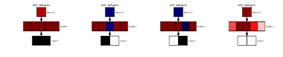
To see all of these activations flow through the network diagram above, you can run through them in the dashboard above.

Or, Conx has a number of methods for visualizing images. In this example below, we get each picture of the network as an “image” and give the list of images to cx.view.

cx.view([net.picture(net.dataset.inputs[i], format="image") for i in range(4)], scale=3.2)

2.3. conx options

2.3.1. Propagation functions

There are five ways to propagate activations through the network:

• Network.propagate(inputs) - propagate these inputs through the network
• Network.propagate_to(inputs) - propagate these inputs to this bank (returns the output at that layer)
• Network.propagate_from(bank-name, activations) - propagate the activations from bank-name to outputs
• Network.propagate_to_image(bank-name, activations, scale=SCALE) - returns an image of the layer activations
• Network.propagate_to_features(bank-name, activations, scale=SCALE) - gets a matrix of images for each feature (channel) at the layer

net.propagate_from("hidden1", [0, 1, 0, 0, 1])

[0.011234397]

net.propagate_to("hidden1", [0.5, 0.5])

[0.0, 0.0, 0.0, 0.2627236843109131, 0.0]

net.propagate_to("hidden1", [0.1, 0.4])

[0.0, 0.0, 0.5568257570266724, 0.0, 0.0]

There is also a propagate_to_image() that takes a bank name, and inputs.

net.propagate_to_image("hidden1", [0.1, 0.4]).resize((500, 100))

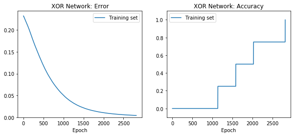
2.3.2. Plotting options

You can re-plot the plots from the entire training history with:

net.plot_results()

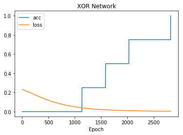
You can plot the following values from the training history:

• “loss” - error measure (eg, “mse”, mean square error)
• “acc” - the accuracy of the training set

You can plot any subset of the above on the same plot:

net.plot(["acc", "loss"])

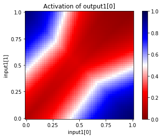
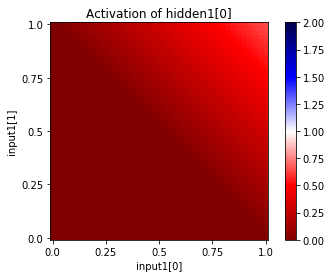
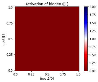
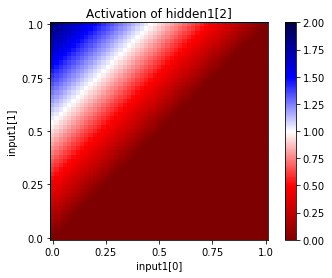
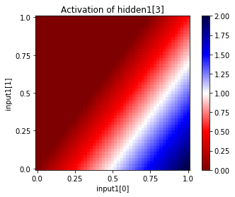
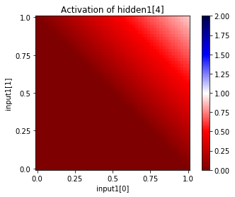
You can also see the activations at a particular unit, given a range of input values for two input units. Since this network has only two inputs, and one output, we can see the entire input and output ranges:

for i in range(net["hidden1"].size):
    net.plot_activation_map(from_layer="input1", from_units=(0,1),
                            to_layer="hidden1", to_unit=i)

net.plot_activation_map(from_layer="input1", from_units=(0,1),
                        to_layer="output1", to_unit=0)